1. 개요
2. Partial Convolution Layer
3. Loss function
4. 코드 구현 및 실험 결과
A. Partial Convolution
B. U-Net
C. Loss 구현
1. Pixel Loss
2. Perceptual Loss, Style Loss
3. Total Variation Loss
D. 실험 결과
1. 개요
Image inpainting이란, 이미지의 손상된 부분을 복원하는 작업을 말합니다.
이 논문 이전의 image inpainting 연구들은 대체로 일반 convolution layer를 사용해 이 문제를 해결해 왔습니다. 그러나 일반 convolution layer는 구멍을 채울 때 convolution filter의 평균 값으로 구멍을 채워넣어 이미지가 흐릿해지는 문제가 있었다고 합니다.

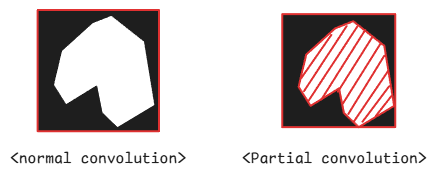
예를 들어 일반 convolution layer를 사용해 위와 같이 구멍이 있는 부분을 살펴본다면, convolution filter가 구멍 픽셀의 정보까지 포함하여 정보를 처리하게 됩니다. 이렇게 되면 모델이 구멍 부분을 예측하는데 필요하지 않은 잘못된 정보가 전달될 수도 있습니다.
이를 해결하기 위해 여러가지 후처리 기법들도 연구되었지만 복잡하고 이를 완전히 해결하는 방법은 아니었습니다.
또 다른 문제점은 기존 연구들은 규칙적인 네모 모양의 구멍을 메꾸는 데만 집중했다는 것입니다. 이는 모델이 네모 모양을 복원하는 데만 overfitting되게 만들어 다른 모양의 구멍에는 힘을 못 쓸 가능성이 높고, 실사용에 제약을 가져올 수 있습니다.
이 논문에서 제시하고자 하는 바는 위 2가지 문제를 해결하는 것입니다.
- Partial Convolution을 사용해 기존 convolution layer의 오작동을 방지한다.
- 불규칙한 모양의 구멍을 예측하는 모델을 학습하여 overfitting을 방지한다.
그럼 지금부터 이 논문에서 어떻게 image inpainting 문제를 해결했는지 확인해 보도록 하겠습니다.
2. Partial Convolution Layer
기존 Convolution layer의 문제점은 모델이 구멍을 복원하는데 도움이 되지 않는 '구멍' 부분의 픽셀 정보를 함께 처리한다는 것이었습니다.
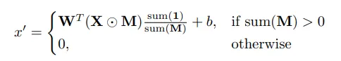
그렇다면 어떻게 이를 해결할 수 있을까요? Partial Convolution은 이 구멍 픽셀의 정보를 아예 무시하는 것으로 해결했습니다.
$$ x'=\left\{\begin{matrix}
W^T(X\bigodot M){\text{sum}(1)\over\text{sum}(M)}+b, & \text{if sum}(M)>0\\
0, & \text{otherwise} \\
\end{matrix}\right. $$
($x$는 input 이미지, $w$와 $b$는 convolution layer의 파라미터)
$M$은 binary mask로, 이미지에서 무시해야 하는 구멍 범위의 픽셀부분을 가리는 mask입니다. 즉, mask 가린 픽셀값이 0인 구멍 부분은 계산에서 아예 제외하고, 나머지 유효한 픽셀 값만 convolution 계산에 포함하는 것이죠.
Partial convolution은 아래와 같이 mask 업데이트를 통해 점차 mask의 크기를 줄여나가며 이미지 복원을 수행하게 됩니다.
논문에서 전체적인 모델 구조는 UNet 구조를 사용했으며, 기존의 UNet과 다른 점은 모든 convolution layer를 Partial convolution 레이어로 대체했다는 것입니다.
3. Loss function
모델 학습을 위해 사용한 loss는 무려 4개나 됩니다. 하나씩 살펴보겠습니다.
($I$는 이미지, $M$은 마스크를 의미합니다.)
($I_{out}$: 모델이 생성한 이미지 / $I_{gt}$: 원본 이미지)
1. Per-pixel losses
원본 이미지와 모델의 예측 이미지 사이의 pixel을 비교하는 loss로, 구멍 부분과 원본 부분의 가중치를 다르게 하여 모델이 구멍 복원에 좀 더 집중할 수 있도록 합니다.
$L_{hole}={1\over N_{I_{gt}}}||(1-M)\bigodot(I_{out}-I_{gt})||_1$
$L_{valid}={1\over N_{I_{gt}}}||(M)\bigodot(I_{out}-I_{gt})||_1$
$(N_{I_{gt}}=C*H*W)$
$L_{hole}$은 구멍 부분의 pixel loss, $L_{valid}$는 구멍이 아닌 부분의 pixel loss입니다. 모두 L1 loss를 사용했습니다.
2. Perceptual Loss
Perceptual Loss는 사전학습된 VGG 모델을 이용해 두 이미지가 서로 얼마나 유사한지를 나타내는 지표입니다. Per-pixel losses와 같이 픽셀 간의 비교만으로는 이미지의 고차원적인 특징(예를 들면 이미지의 경계, 텍스처, 패턴 등)을 비교하기 어렵습니다. 따라서 이미지에 대해 어느정도 지각 능력을 갖고 있는 사전학습된 VGG 모델을 이용해 두 이미지가 정말 유사한지를 한번 더 비교하는 것입니다.
본 논문에서는 사전학습된 VGG-16 모델을 사용했으며, VGG 레이어의 중간 레이어인 pool1, pool2, pool3 레이어의 output을 서로 비교했다고 합니다. (자세한건 아래 코드 구현에서 설명하겠습니다.)
$$L_{perceptual}=\sum^{P-1}_{p=0}{||\Psi^{I_{out}}_p-\Psi^{I_{gt}}_p||_1\over N_{\Psi^{I_{gt}}_p}}+\sum^{P-1}_{p=0}{||\Psi^{I_{comp}}_p-\Psi^{I_{gt}}_p||_1\over N_{\Psi^{I_{gt}}_p}}$$
$\Psi$는 VGG 모델을 의미하며, 모델이 예측한 이미지의 vgg output($\Psi_p^{I_{out}}$)과 원본 이미지의 vgg output ($\Psi_p^{I_{gt}}$) 를 비교한 loss(왼쪽 항)와 comp 이미지의 vgg output($\Psi_p^{I_{comp}}$) 과 원본 이미지의 vgg output ($\Psi_p^{I_{gt}}$)을 비교한 loss(오른쪽 항)을 더해주면 됩니다. 비교에는 L1 distance를 사용합니다.
여기서 comp 이미지란, 구멍 부분만 비교하기 위해 만들어진 이미지를 말합니다. comp 이미지는 $I_{out}$에서 구멍 부분을 뺀 나머지 부분을 $I_{gt}$로 대체한 이미지입니다. 즉, 원본 이미지와 구멍 부분의 픽셀값만 다른 이미지입니다.
분모의 $N_{\Psi^{I}_p}$는 정규화를 위한 상수로 vgg output의 차원 수의 곱을 의미합니다.
3. Style loss
Style loss는 Perceptual Loss와 유사하게 VGG 모델을 사용하지만, 두 이미지에서 특정한 패턴이 똑같이 나타나는지를 측정하기 위한 지표입니다.
Perceptual Loss와 같이 vgg output을 사용하며, 두 이미지의 vgg output 사이의 L1 distance를 측정하기 전에 gram matrix를 적용합니다. gram matrix는 입력 feature의 서로 다른 위치 사이의 내적을 계산하는 수식으로 아래와 같이 계산됩니다.
$$\text{Gram_Matrix}=F\cdot F^T$$
Gram matrix를 적용한 style loss의 수식은 아래와 같습니다.
$L_{style_{out}}=\sum^{P-1}_{p=0}{1\over C_pC_p}||K_p((\Psi^{I_{out}})^T(\Psi^{I_{out}}_p)-(\Psi^{I_{gt}}_p)^T(\Psi^{I_{gt}}_p))||_1$
$L_{style_{comp}}=\sum^{P-1}_{p=0}{1\over C_pC_p}||K_p((\Psi^{I_{comp}})^T(\Psi^{I_{comp}}_p)-(\Psi^{I_{gt}}_p)^T(\Psi^{I_{gt}}_p))||_1$
$K_P$는 (${1\over C_pH_pW_p$), $C_P$는 VGG output의 채널값으로 정규화를 위한 상수입니다.
4. Total variation Loss (TV Loss)
마지막으로 tv loss입니다. tv loss는 바로 인접한 픽셀 간의 차이값을 계산해 이미지가 더 부드럽게 생성되도록 하는 loss입니다.
$$L_{tv}=\sum_{(i,j)\in R,(i,j+1)\in R}{||I^{i,j+1}_{comp}-I^{i,j}_{comp}||_1\over N_{I_comp}}+\sum_{(i,j)\in R,(i+1,j)\in R}{||I^{i+1,j}_{comp}-I^{i,j}_{comp}||_1\over N_{I_comp}}$$
$R$은 이미지의 픽셀 좌표를 담는 행렬로, 각 픽셀마다 바로 옆의 픽셀 값과 비교하여 그 차이가 크지 않도록 규제합니다. 위 loss를 통해 모델이 보다 부드러운 이미지를 생성할 수 있게 됩니다.
이렇게 4개의 loss를 모두 합치면 이 모델의 최종 loss가 완성됩니다.
$$L_{total}=L_{valid}+6L_{hole}+0.05L_{perceptual}+120(L_{style_{out}}+L_{style_{comp}})+0.1L_{tv}$$
각 loss마다 가중치도 위와 같이 따로 적용하여 모델이 더 안정적으로 수렴하도록 합니다.
4. 코드 구현 및 실험 결과
저는 이 논문의 코드를 PyTorch를 사용해 구현해 보았습니다. 코드는 아래 링크에서 확인할 수 있습니다.
GitHub - intrandom5/Image-inpainting-for-irregular-holes-using-partial-convolutions: Implementation of 'Image Inpainting for Irr
Implementation of 'Image Inpainting for Irregular holes using Partial Convolutions. - intrandom5/Image-inpainting-for-irregular-holes-using-partial-convolutions
github.com
코드 구현은 chatGPT와 아래 링크의 도움을 받았습니다.
https://github.com/MathiasGruber/PConv-Keras/blob/master/libs/pconv_layer.py
실험 데이터셋은 아래 링크의 데이터를 사용했습니다.
https://dacon.io/competitions/official/236420/data
이미지 색상화 및 손실 부분 복원 AI 경진대회 - DACON
분석시각화 대회 코드 공유 게시물은 내용 확인 후 좋아요(투표) 가능합니다.
dacon.io
A. Partial Convolution
우선 Partial Convolution의 구현 코드부터 살펴보겠습니다.
class PartialConv2d(nn.Module):
    def __init__(self, in_channels, out_channels, kernel_size, stride=1, padding=0):
        super(PartialConv2d, self).__init__()
        self.kernel_size = kernel_size
        self.input_conv = nn.Conv2d(in_channels, out_channels, kernel_size, stride, padding)
        self.mask_conv = nn.Conv2d(in_channels, out_channels, kernel_size, stride, padding, bias=False)
        nn.init.constant_(self.mask_conv.weight, 1.0)  # Initialize mask conv weights to 1
        self.mask_conv.weight.requires_grad = False  # Freeze mask conv weights

    def forward(self, x, mask):
        # Convolution on input
        img_out = self.input_conv(x * mask)

        # Update mask
        with torch.no_grad():
            mask_out = self.mask_conv(mask)
            mask_out = torch.clamp(mask_out, 0, 1)

        mask_ratio = self.kernel_size**2 / (mask_out + 1e-8)
        mask_ratio = mask_ratio * mask_out

        img_out = img_out * mask_ratio  # Ensure the output is zero where mask is zero

        return img_out, mask_out
보면 이미지와 더불어 mask도 함께 입력 받는 것을 알 수 있습니다. mask를 다루는 convolution 레이어는 학습되지 않으며, 최종적으로 img_out에 곱해져 mask 부분의 값이 0이 되도록 합니다.
B. U-Net
U-Net은 오토인코더 구조로, 인코더의 출력이 디코더의 입력으로 concatenate 되어 이미지의 복원에 도움을 주는 구조입니다. 본 논문의 모델은 기존의 convolution layer를 partial convolution으로 바꿔주기만 하면 됩니다. (이와 더불어 partial convolution은 mask도 처리하기 때문에 mask에 관한 처리도 추가적으로 해줘야 합니다.)
우선 U-Net을 구성하는 기본적은 convolution block 코드입니다.
class ConvBlock(nn.Module):
    def __init__(self, in_channels, out_channels):
        super(ConvBlock, self).__init__()
        self.partial_conv1 = PartialConv2d(in_channels, out_channels, kernel_size=3, padding=1)
        self.batch_norm1 = nn.BatchNorm2d(out_channels)
        self.relu1 = nn.ReLU(inplace=True)
        self.partial_conv2 = PartialConv2d(out_channels, out_channels, kernel_size=3, padding=1)
        self.batch_norm2 = nn.BatchNorm2d(out_channels)
        self.relu2 = nn.ReLU(inplace=True)

    def forward(self, x, mask):
        x, mask = self.partial_conv1(x, mask)
        x = self.batch_norm1(x)
        x = self.relu1(x)
        x, mask = self.partial_conv2(x, mask)
        x = self.batch_norm2(x)
        x = self.relu2(x)
        return x, mask
일반 convolution layer 대신에 앞서 구현한 partial convolution 레이어를 사용했으며, mask 업데이트를 위해 mask를 추가적으로 입력 받고, mask를 추가적으로 출력합니다.
다음은 디코더 블록입니다. 인코더와 달리 concatenate도 수행해야 하기 때문에 디코더 block은 클래스를 따로 만들었습니다.
def crop_and_concat(upsampled, bypass):
    _, _, h, w = upsampled.size()
    bypass_cropped = center_crop(bypass, [h, w])
    return torch.cat((upsampled, bypass_cropped), dim=1)

class DecoderBlock(nn.Module):
    def __init__(self, in_channels, out_channels):
        super(DecoderBlock, self).__init__()
        self.decoder = ConvBlock(in_channels, out_channels)
        self.convert_channel = nn.Conv2d(in_channels, out_channels, kernel_size=1, padding='same')

    def forward(self, img_in, mask_in, img_enc, mask_enc):
        dec = F.interpolate(img_in, scale_factor=2, mode='nearest')
        dec = self.convert_channel(dec)
        dec = crop_and_concat(dec, img_enc)
        d_mask = F.interpolate(mask_in, scale_factor=2, mode='nearest')
        d_mask = self.convert_channel(d_mask)
        d_mask = crop_and_concat(d_mask, mask_enc)
        dec, d_mask = self.decoder(dec, d_mask)
        return dec, d_mask
논문을 따라 interpolate를 수행해 feature의 크기를 늘려주었습니다. 그 뒤에 인코더의 출력(img_enc)과 채널 수를 맞추기 위해 1x1 convolution을 수행해 채널 수를 변경해준 뒤, img_enc와 concat해줬습니다.
마지막으로 U-Net 본체 코드입니다.
class UNet(nn.Module):
    def __init__(self, in_channels=1, out_channels=3, start_dim=64):
        super(UNet, self).__init__()
        # Encoder layers
        self.encoder1 = ConvBlock(in_channels, start_dim)
        self.encoder2 = ConvBlock(start_dim, start_dim * 2)
        self.encoder3 = ConvBlock(start_dim * 2, start_dim * 4)
        self.encoder4 = ConvBlock(start_dim * 4, start_dim * 8)

        # Bottleneck
        self.bottleneck = ConvBlock(start_dim * 8, start_dim * 16)

        # Decoder layers
        self.decoder4 = DecoderBlock(start_dim * 16, start_dim * 8)
        self.decoder3 = DecoderBlock(start_dim * 8, start_dim * 4)
        self.decoder2 = DecoderBlock(start_dim * 4, start_dim * 2)
        self.decoder1 = DecoderBlock(start_dim * 2, start_dim)

        # Final output layer
        self.final = PartialConv2d(start_dim, out_channels, kernel_size=1)

    def forward(self, x, mask):
        # Encoder
        enc1, e_mask1 = self.encoder1(x, mask)
        enc2, e_mask2 = self.encoder2(F.max_pool2d(enc1, 2), F.max_pool2d(e_mask1, 2))
        enc3, e_mask3 = self.encoder3(F.max_pool2d(enc2, 2), F.max_pool2d(e_mask2, 2))
        enc4, e_mask4 = self.encoder4(F.max_pool2d(enc3, 2), F.max_pool2d(e_mask3, 2))

        # Bottleneck
        bottleneck, mask_bottleneck = self.bottleneck(F.max_pool2d(enc4, 2), F.max_pool2d(e_mask4, 2))

        # Decoder
        dec4, d_mask4 = self.decoder4(bottleneck, mask_bottleneck, enc4, e_mask4)
        dec3, d_mask3 = self.decoder3(dec4, d_mask4, enc3, e_mask3)
        dec2, d_mask2 = self.decoder2(dec3, d_mask3, enc2, e_mask2)
        dec1, d_mask1 = self.decoder1(dec2, d_mask2, enc1, e_mask1)

        # Final output
        output, mask_output = self.final(dec1, d_mask1)
        return output
인코더와 디코더 블록을 4개씩 사용했으며, 각 블록마다 feature의 크기가 절반씩 줄어들고 늘어납니다.
C. Loss 구현
Loss가 꽤 많기 때문에 클래스로 따로 구현했습니다.
class PartialUNetLoss(nn.Module):
    def __init__(self, loss_weights, device):
        super().__init__()
        self.vgg = vgg16(weights="IMAGENET1K_V1").features[:17]
        self.vgg = torch.nn.ModuleList(self.vgg)
        self.vgg.to(device)
        if type(loss_weights) == str:
            loss_weights = eval(loss_weights)
        self.loss_weights = loss_weights
사전학습된 vgg16 모델을 불러왔으며, pool1, pool2, pool3 레이어만 사용하기 때문에 17번째 레이어까지만 불러왔습니다.
loss_weights는 [1, 6, 0.05, 120, 0.1]의 값을 담고 있는 리스트로, 논문에서 설정한 가중치와 똑같이 설정했습니다.
1. Pixel Loss
가장 쉬운 pixel loss의 경우 아래와 같이 구현하면 됩니다. 구멍 부분과 구멍이 아닌 부분을 나눠서 계산합니다.
# pixel loss
valid_loss = F.l1_loss(pred_img*mask, target_img*mask)
hole_loss = F.l1_loss(pred_img*(1-mask), target_img*(1-mask))
2. Perceptual Loss, Style Loss
다음으로 perceptual loss와 style loss를 계산하기 위해 모델이 예측한 이미지(pred_img), 원본 이미지(target_img), 구멍 부분 비교를 위한 이미지(comp_img)로부터 각각 vgg feature를 뽑아냅니다.
    def vgg_pooling(self, x):
        with torch.no_grad():
            pooling_idx = [4, 9, 16]
            pooling_outputs = []
            for i, layer in enumerate(self.vgg):
                x = layer(x)
                if i in pooling_idx:
                    pooling_outputs.append(x)
        return pooling_outputs

    ...

        # vgg pooling
        tgt_pools = self.vgg_pooling(target_img)
        out_pools = self.vgg_pooling(pred_img)
        comp_pools = self.vgg_pooling(comp_img)
pool1, pool2, pool3 레이어는 각각 vgg의 4번째 9번째 16번째 레이어를 말합니다. 각 레이어의 output을 리스트에 담아 출력해 줬습니다.
    def remove_inf_nan(self, x):
        x[x!=x]=0
        x[~torch.isfinite(x)]=0
        return x

    def gram_matrix(self, x):
        x = torch.clamp(x, -1e3, 1e3)  # 값 제한
        b, c, w, h = x.size()
        features = x.view(b, c, -1)
        gram = torch.bmm(features, features.transpose(1, 2))
        gram = gram / (c * h * w + 1e-8)
        return self.remove_inf_nan(gram)

    def get_vgg_loss(self, tgt_pools, out_pools, comp_pools):
        perceptual_loss = 0
        style_loss = 0
        for tgt, out, comp in zip(tgt_pools, out_pools, comp_pools):
            perceptual_loss += F.l1_loss(out, tgt)
            perceptual_loss += F.l1_loss(comp, tgt)
            out_gram = self.gram_matrix(out)
            tgt_gram = self.gram_matrix(tgt)
            style_loss += F.l1_loss(out_gram, tgt_gram)
        return perceptual_loss, style_loss
각 vgg 레이어의 출력물들(tgt, out, comp)로부터 perceptual loss와 style loss를 각각 계산합니다. gram_matrix의 경우 mixed-precision으로 학습할 때 계산값이 폭주하는 경우가 자주 발생해 이를 방지하기 위한 코드 (clamp나 remove_inf_nan 메소드)가 추가되었습니다.
3. Total variation Loss
    def total_variation_loss(self, mask, y_comp):
        # Dilate the mask
        kernel = torch.ones((1, 1, 3, 3), device=mask.device)  # 3x3 kernel
        if mask.shape[1] == 3:
            mask = mask[:, :1, :, :]
        dilated_mask = F.conv2d(1 - mask, kernel, padding=1)

        # Threshold the dilated mask to create binary values
        dilated_mask = (dilated_mask > 0).float()

        # Apply dilated mask to y_comp
        P = dilated_mask * y_comp

        # Calculate total variation loss within the masked area
        dh = P[:, :, 1:, :] - P[:, :, :-1, :]
        dw = P[:, :, :, 1:] - P[:, :, :, :-1]
        tv_loss = torch.sum(torch.abs(dh)) + torch.sum(torch.abs(dw))
        valid_pixels = torch.sum(dilated_mask) + 1e-8

        return tv_loss / valid_pixels
솔직히 tv loss의 구현은 저도 세세하게 이해하기는 힘들었습니다. 하지만 직관적으로는 모든 픽셀을 하나씩 미룬 이미지와 일반 이미지 사이의 차이를 비교(dh와 dw)한 뒤, 그 차이를 tv_loss에 담은 뒤, 유효한 픽셀 수로 나눠 최종적으로 tv_loss를 출력한다고 이해했습니다.
D. 실험 결과


위 코드로 5에포크 학습해 본 결과, 결과는 위와 같이 나타났습니다. 평가 지표로는 영상의 화질 손실량을 평가하는 SSIM을 사용했습니다.
학습 그래프를 보면 모델이 아직 완전히 수렴하지 않은 상태입니다. 전 자원의 한계로 이정도만 학습하고 멈췄지만, 더 학습한다면 더 좋은 결과를 낼 수 있을 것으로 예상됩니다.
'딥러닝 논문리뷰' 카테고리의 다른 글
| [논문 리뷰] DeepSeek-V3: Technical Report (0) | 2025.02.13 |
|---|---|
| [EEVE] Efficient and Effective Vocabulary Expansion Towards Multilingual Large Language Models (1) | 2024.05.02 |
| Textbooks are all you need (phi-1) (1) | 2024.01.17 |
| 구글의 BARD와 openAI의 ChatGPT는 어떻게 다를까? (1) | 2023.12.20 |
| FASTSPEECH 2: FAST AND HIGH-QUALITY END-TOEND TEXT TO SPEECH (1) | 2023.10.29 |


